Fuzzy time series
A fuzzy time series (FTS) model forecasts a numeric series by describing it with words. Instead of "enrollment was 15 460", the model says "enrollment was A3". It learns which word tends to follow which, and turns the predicted word back into a number. The idea goes back to Song and Chissom (1993). ferrifuzz implements the simple and widely taught method of Chen (1996), in first-order and high-order form.
FTS models are small and transparent: the whole model is a short list of rules such as "after A2 comes A2 or A3". They are a good baseline for short series where a statistical model would overfit.
The method, step by step
1. Define the universe
Take the range of the training data and pad it by a margin (a fraction of the range, 10 %
by default) on each side:
You can also set the universe yourself with universe=(lo, hi). This is useful when you know
the physical limits of the quantity, or when the test data will go beyond the training range.
2. Partition it into fuzzy sets
Split into n_partitions evenly spaced, overlapping fuzzy sets .
Neighbouring sets cross at 0.5:
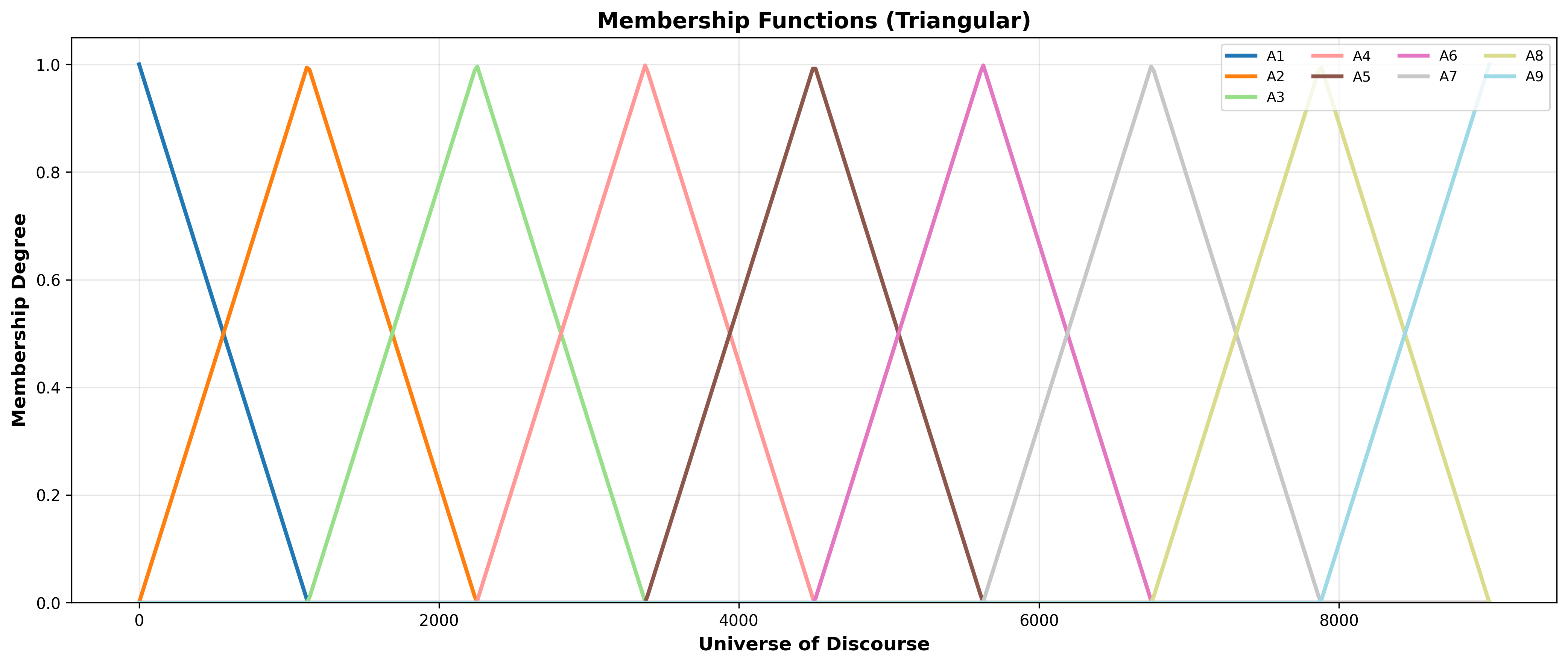
mf_type picks the partition shape: "triangle" (default) or "gaussian". Any other value
is an error.
3. Fuzzify the series
Replace each value with the partition where its membership is highest. Ties go to the lower partition.
Values outside the universe map to the nearest partition: below the universe,
above it. A NaN (or infinite) value in the training series makes fit raise ValueError, so fill or
drop missing values first.
4. Build fuzzy logical relationships
Each consecutive pair gives a fuzzy logical relationship (FLR) : "after came ". FLRs with the same left-hand side are merged into a fuzzy logical relationship group (FLRG). Repeated consequents are counted once:
5. Forecast
To forecast the value after a point fuzzified as , look up the FLRG of and average the centers of its consequents:
If never appeared on the left-hand side during training, there is no FLRG. The model then falls back to , the center of itself ("no change").
First order vs high order
A first-order model (order=1) only looks at the last value. An order- model
uses the last fuzzified values as the antecedent: .
Higher orders can tell apart situations such as "rising into A3" and "falling into A3", but
each antecedent is seen fewer times, so the model needs more data. With many partitions and
a high order, the model can simply memorise a short training series. Always evaluate on data
the model has not seen.
Worked example
from ferrifuzz.fts import FuzzyTimeSeries

series = [10, 12, 14, 13, 15, 17, 16, 18, 20, 19, 21, 23]
model = FuzzyTimeSeries(n_partitions=5, order=1).fit(series)

print(model.summary())
for p in model.get_partitions():
    print(p)
for g in model.get_flrgs():
    print(g)
FuzzyTimeSeries(n_partitions=5, order=1, mf_type='triangle', fitted, 4 FLRGs)
  Universe    : [8.7000, 24.3000]
  Partitions  : 5  (triangle)
  FLRGs found : 4
Partition('A1', center=8.7000)
Partition('A2', center=12.6000)
Partition('A3', center=16.5000)
Partition('A4', center=20.4000)
Partition('A5', center=24.3000)
FLRG(A1 -> A2)
FLRG(A2 -> A2, A3)
FLRG(A3 -> A3, A4)
FLRG(A4 -> A4, A5)
The range is 13, so the margin of 1.3 gives the universe . The series fuzzifies
to A1 A2 A2 A2 A3 A3 A3 A3 A4 A4 A4 A5. FLRGs print 0-based partition indices, so
(1,) → [1, 2] means .
One-step-ahead forecasts (aligned with series[1:]):
model.forecast(series)
# [12.6, 14.55, 14.55, 14.55, 18.45, 18.45, 18.45, 18.45, 22.35, 22.35, 22.35]
After an A2 the forecast is . Forecasting past the end:
model.predict(series[-1:], steps=3) # [24.3, 24.3, 24.3]
The last value, 23, is A5. A5 never appeared on the left of an FLR, so the model falls back to the center of A5 and stays there.
Chen's forecasts can only take a small set of values (averages of partition centers), so the forecast curve is a staircase. More partitions give finer steps, but each FLRG is then seen fewer times.
Scoring
model.evaluate(series) forecasts one step ahead over series, aligns the forecasts with
series[order:] and returns RMSE, MAE and MAPE:
model.evaluate(series) # {'rmse': 1.58, 'mae': 1.31, 'mape': 7.71}
This is the same as calling ferrifuzz.metrics.score yourself:
from ferrifuzz.metrics import score

score(series[model.order:], model.forecast(series))
Always compare against the naive forecast . On smooth series it is hard to beat, and an FTS model that loses to it has learned nothing useful.
In ferrifuzz
- Python:
ferrifuzz.fts,ferrifuzz.metrics - Rust:
ferrifuzz::fts,ferrifuzz::metrics - Tutorial: Forecasting university enrollment
Further reading
- Q. Song and B. S. Chissom, "Fuzzy time series and its models", Fuzzy Sets and Systems, 1993.
- S.-M. Chen, "Forecasting enrollments based on fuzzy time series", Fuzzy Sets and Systems, 1996.